Now let's see how we can combine determiners and nouns into NPs. This is a slightly complex but very interesting rule, as it takes care both of the correct binding of a variable bound by a quantifier, and of the introduction of the dominance edges we need in order to represent scope ambiguities.

The rule looks as follows:

combine(np1:NP,[det:DET,n2:N]) :-
        DET = usr([DETRoot|_],_,_,_),
        N = usr([NRoot|_],_,_,_),
        NewUsr = usr(
        [Root,N1,N2,N3,N4],
        [N1:(N2@N3),N2:(DETRoot@NRoot),N3:lambda(N4),Root:var],
        [dom(N4,Root)],
        [bind(Root,N3)]),
        mergeUSR(merge(NewUsr,merge(DET,N)),NP).

Again, this becomes more readable when written as a constraint graph:

The root of an NP is a var-node.

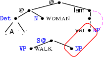
The root of the constraint graph for the entire NP is the node Root, i.e. the node which is labeled with var. Although this may seem a bit counterintuitive, it is extremely useful considering how the NP will later combine with a VP (see Section ``''). The VP semantics will be applied to the root of the NP graph. That is, the verb semantics will be applied to a variable that is bound by the quantifier -- exactly what we want! Consider the constraint for ``a woman walks'' given below. We show the last step of semantics construction and one parent normalization step.

and before unification...	...after unification.

...after normalization.

Look at the leftmost graph. On top you see the representation of an NP as discussed above. Here, the representation of the determiner (abbreviated in the figure) and the noun representation have already been integrated (by unification). Below you can see the representation of an S where the VP has already been found. The next (and last) step in semantics construction is the integration of the NP into the S, i.e. the unification of the root node of the NP and the NP node of the S.

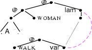
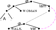
The result of this unification can be seen in the middle graph. This constraint graph is the underspecified representation for the sentence ``a woman walks''. With the help of one simple parent normalization step, we end up with the solved form of this graph which can be seen on the right. A minimal solution hereof is the following -expression:

which probably looks much more familiar to you. Now we can now fully realize just how convenient binding constraints are. We can simply relate the variable and its binder within a single semantics construction rule; they are connected forever with an unbreakable link, and we don't have to think at all about variable naming. We could unify both NP nodes in the example above and got (we christened the variable represented by in the -expression given above). If the NP is a proper name as in ``John walks'', the same mechanism unifies the NP node of the sentence with as we have seen in Section ``''. Finally, the remaining dominance edge from in the solved form is one of those dominance edges that can lead to the representation of a scope ambiguity in other configurations. Next, you can see this example with fully expanded determiner.